SVD

Import libraries

Start by importing pytorch & matplotlib. I could not make the latex interpreter work in binder, so the corresponding lines are commented out.

Code

import torch 
import matplotlib.pyplot as plt

Create the functions

The separability proprieties of several functions are investigated. This code first shows the separability proprieties of different ways of clustering the 1D space into two regions. Two types of functions are used to do so: * A sharp step function (Heaviside), * A smooth one (Tanh).

In both cases the position of the jump is parametrised by a scalar parameter \(\alpha\).

Furhter investigations are conducted on moving front(s) with a * A gaussian function that is moving * Two gaussian functions moving at different rates

Code

L = 10                                      # Space domain
Alpha_vect = torch.linspace(0,1,1500)       # vector of alphas
x_vect = torch.linspace(0,L,2000)           # vector of x


Function = 'Heaviside'                      # Alpha-parameterised step function
Function = 'Tanh'                           # smooth alpha-parameterised step function
# Function = 'Gauss'                        # Alpha-parameterised front function
Function = 'Gauss_sum'                      # Double alpha-parameterised front functions




if Function == 'Heaviside':
    F = torch.heaviside((x_vect[:,None] - (1-Alpha_vect[None,:])*L), x_vect[-1]/x_vect[-1])
elif Function == 'Tanh':
    F = torch.tanh((x_vect[:,None] - (1-Alpha_vect[None,:])*L))
elif Function == 'Gauss':
    F = torch.exp(-(x_vect[:,None] - (1-Alpha_vect[None,:])*L)**2)

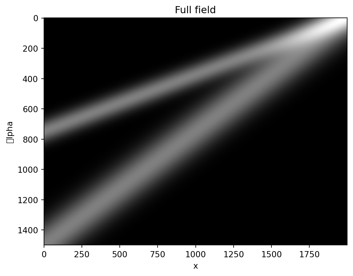
elif Function == 'Gauss_sum':
    F = torch.exp(-(x_vect[:,None] - (1-Alpha_vect[None,:])*L)**2) + torch.exp(-(x_vect[:,None] - (1-2*Alpha_vect[None,:])*L)**2)

Plot the reference function

Code

plt.imshow(F.t(),cmap='gray')
plt.title('Full field')
plt.xlabel('x')
plt.ylabel('\alpha')
# plt.savefig('../Results/FullField_'+Function+'.pdf', transparent=True)  
plt.show()

/Users/daby/anaconda3/lib/python3.11/site-packages/IPython/core/pylabtools.py:152: UserWarning:

Glyph 7 () missing from current font.

Compute its SVD

Code

U, S, V = torch.svd(F)

Compute the truncated function

Code

N = 15                                                  # Number of modes kept for the truncation                   

F_truncated = U[:,:N]@torch.diag(S[:N])@V[:,:N].t()     # Truncated function

Plot the truncated function

Code

plt.imshow(F_truncated.t(),cmap='gray')
plt.title(f'Truncated field, N={N}')
plt.xlabel('x')
plt.ylabel('alpha')
# plt.savefig(f'../Results/TruncatedField_{N}_'+Function+'.pdf', transparent=True)  
plt.show()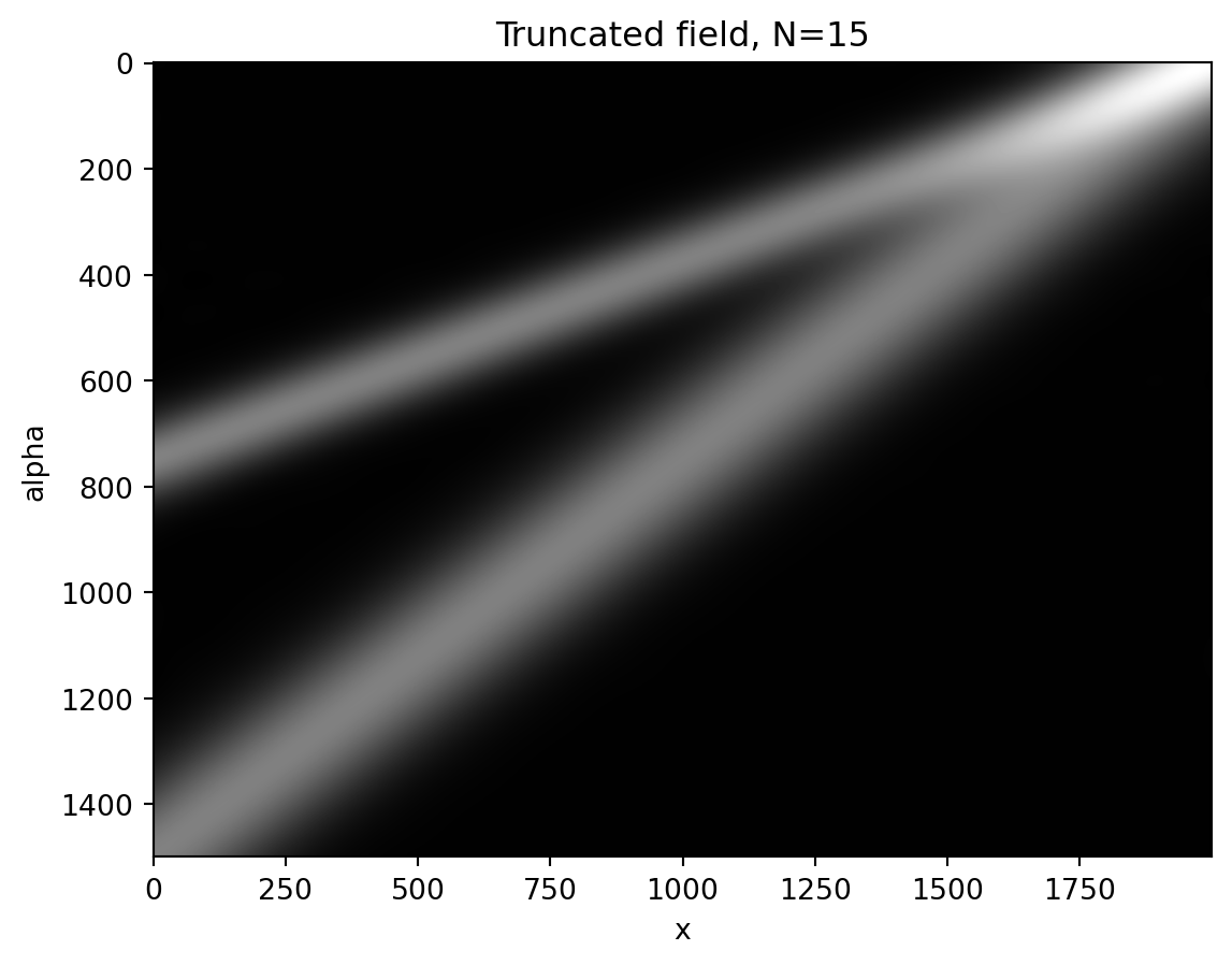

Comparison

The truncated function and its reference are compared for two values * \(\alpha = 1/3\) & * \(\alpha = 2/3\).

Code

plt.plot(x_vect,F[:,1000],'k',label='Full, alpha = 2/3')
plt.plot(x_vect,F_truncated[:,1000],'--',label='Truncated, alpha = 2/3')
plt.plot(x_vect,F[:,500],'k',label='Full, alpha = 1/3')
plt.plot(x_vect,F_truncated[:,500],'--',label='Truncated, alpha = 1/3')
plt.legend(loc="upper left")
plt.title(f'2 slices of the field, N={N}')
plt.xlabel('x')
plt.ylabel('f(x,alpha)')
# plt.savefig(f'../Results/Sliced_TruncatedField_{N}_'+Function+'.pdf', transparent=True)  
plt.show()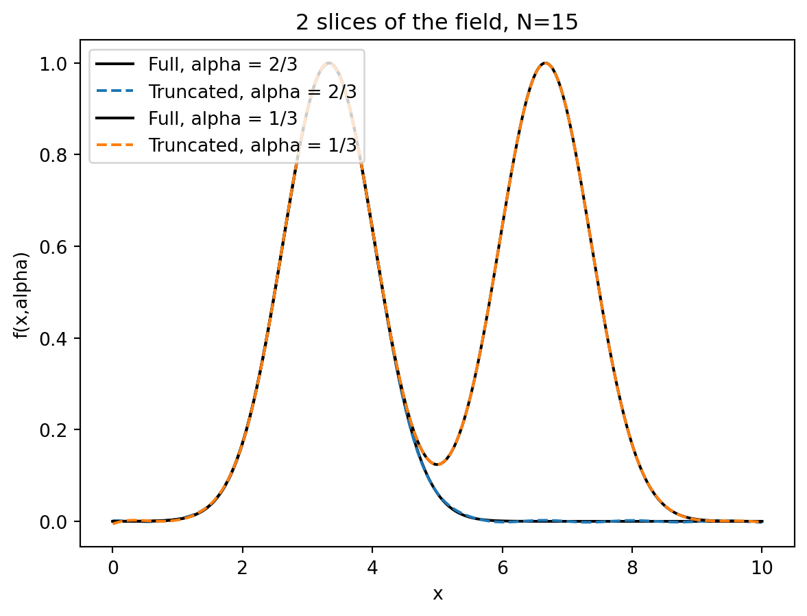

Interactive plot comparing the truncated function and the reference

This interactive plot allows to change the number of modes in the truncation and the value of the parameter \(\alpha\) .

Code

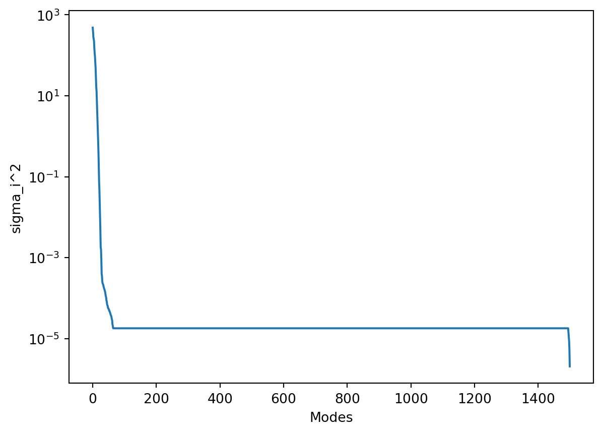
plt.semilogy(S)
plt.ylabel('sigma_i^2')
plt.xlabel('Modes')
# plt.savefig(f'../Results/SVD_Decay_'+Function+'.pdf', transparent=True)  
plt.show()