Non-linear manifold learning

SVD

This section focuses on using using the SVD to find a linear subspace of lower dimension in which to project the data. The objective is to show that dimensionality reduction works well in linear subspaces when the underlying structure is linear but quickly shows limitation for non-linear structures.

Application to a noisy affine function

We first apply the SVD to an affine functions. The physical space of the dataset is \(\mathbb{R}^2\) but the data set is in fact 1D. The SVD is used to find a suitable 1D linear subspace of \(\mathbb{R}^2\) in which the data can be projected without loosing any information.

Function definition and SVD computation

We start by defining the function and by computing the SVD of all the 2D snapshots.

Code

import numpy as np
import matplotlib.pyplot as plt

Code

n_sample = 100                                                                              # Choose number of samples
x = np.linspace(0,10,n_sample)                                                              # create vector x

# Affine parameters
a = 1.5                                                                                     # Slope
b=0                                                                                         # y-axis origin

# Affine function
y = a*x+b                                                                                   # Affine function
X = np.stack((x,y))                                                                         # Create numpy array

# Noise
n_coef = 1                                                                                  # Noise magnitude
X += + n_coef*np.random.rand(*X.shape)                                                      # Noisy data

# SVD
U,S,V = np.linalg.svd(X)                                                                   # SV Decomposition

Plots

To visualise the underlying space found in the data by the SVD, we plot the principal directions \(\nu_1\) and \(\nu_2\) onto the initial dataset.

Code

colors_1D = plt.cm.viridis(np.linspace(0, 1, len(X[0,:])))                                        # Generate a color gradient

# plots
# Origin point
origin = np.array([[0, 0], [0, 0]]) 
U_scaled = -5*U
plt.figure(figsize=(6, 6))
# plt.quiver(*origin, U_scaled[:, 0], U_scaled[:, 1], angles='xy', scale_units='xy', scale=1, color=['r', 'b'])
plt.quiver(*origin, U_scaled[0, 0], U_scaled[0, 1], angles='xy', scale_units='xy', scale=1, color='#01426A', label=r'$\nu_1$')
plt.quiver(*origin, U_scaled[1, 0], U_scaled[1, 1], angles='xy', scale_units='xy', scale=1, color='#CE0037', label=r'$\nu_2$')
plt.legend()
plt.gca().set_aspect('equal')
plt.ylim(-4, 15)
plt.xlim(-4, 15)
plt.xlabel(r"$x$")
plt.ylabel(r"$y$")
# plt.plot(X[0,:],X[1,:],'+')
# plt.scatter(X[0,:],X[1,:], color=colors_1D, s=100)           
plt.scatter(X[0,:],X[1,:], facecolors='none', edgecolors=colors_1D, s=100)             

plt.title("Principal component base and data points")
plt.show()
plt.close()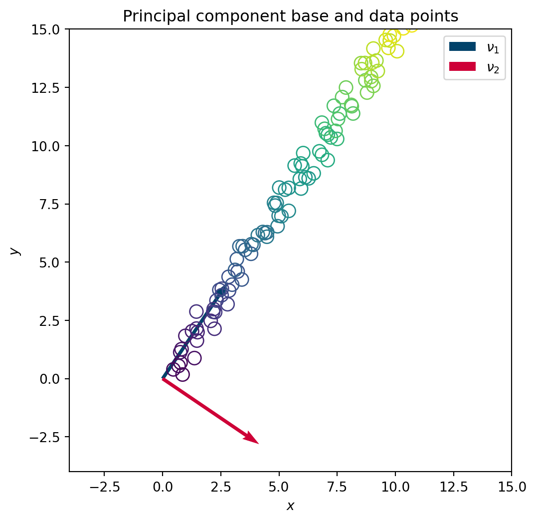

We then project the data onto the latent space \(\left(\nu_1,\nu_2\right)\).

Code

# in the latent space

X_tilde = np.transpose(U)@X
# plt.plot(X_tilde[0,:],X_tilde[1,:],"-o")
plt.scatter(X_tilde[0,:],X_tilde[1,:], color=colors_1D, s=100)           

plt.gca().set_aspect('equal', adjustable='box')
plt.xlabel(r"$\nu_1$")
plt.ylabel(r"$\nu_2$")
plt.show()
plt.close()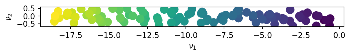

We can see that the initial 2D data in fact lies in a 1D space and that the first principal direction \(\nu_1\) is sufficient to describe the full data set.

Application to non-linear function

To show the limitation of the SVD to find non-linear manifold, a sin function is now studied in a similar manner.

Function definition and SVD computation

Again, we start by defining the function and by computing the SVD of all the 2D snapshots.

Code

# In 1D for an sin function


n_sample = 100                                                                              # Choose number of samples
# x = np.linspace(0,np.pi/4,n_sample)
x = np.linspace(0,6,n_sample)                                                               # create vector x

# Affine parameters
a = 1.5                                                                                     # Slope
b=0                                                                                         # y-axis origin

# Affine function
y = np.sin(x)                                                                               # Sin function
X = np.stack((x,y))                                                                         # Create numpy array

# Noise
n_coef = 0.1                                                                                  # Noise magnitude
X += + n_coef*np.random.rand(*X.shape)                                                      # Noisy data

# SVD
U,S,V = np.linalg.svd(X)                                                                   # SV Decomposition

Plots

In a similar manner, we plot the principal directions \(\nu_1\) and \(\nu_2\) onto the data set

Code

# plots


# Origin point
origin = np.array([[0, 0], [0, 0]]) 
U_scaled = -5*U
plt.figure(figsize=(6, 6))
# plt.quiver(*origin, U_scaled[:, 0], U_scaled[:, 1], angles='xy', scale_units='xy', scale=1, color=['r', 'b'])
plt.quiver(*origin, U_scaled[0, 0], U_scaled[0, 1], angles='xy', scale_units='xy', scale=1, color='#01426A', label=r'$\nu_1$')
plt.quiver(*origin, U_scaled[1, 0], U_scaled[1, 1], angles='xy', scale_units='xy', scale=1, color='#CE0037', label=r'$\nu_2$')
plt.legend()
plt.gca().set_aspect('equal')
# plt.ylim(-4, 15)
# plt.xlim(-4, 15)
plt.xlabel(r"$x$")
plt.ylabel(r"$y$")
# plt.plot(X[0,:],X[1,:],'+')
plt.scatter(X[0,:],X[1,:], facecolors='none', edgecolors=colors_1D, s=100)             

plt.title("Principal component base and data points - sin")
plt.show()
plt.close()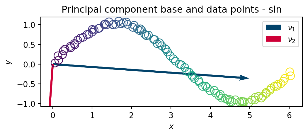

And we project the data onto the latent space \(\left(\nu_1,\nu_2\right)\).

Code

# in the latent space

X_tilde = np.transpose(U)@X
# plt.plot(X_tilde[0,:],X_tilde[1,:],"-o")
plt.scatter(X_tilde[0,:],X_tilde[1,:], color=colors_1D, s=100)           

plt.gca().set_aspect('equal', adjustable='box')
plt.xlabel(r"$\nu_1$")
plt.ylabel(r"$\nu_2$")
plt.show()
plt.close()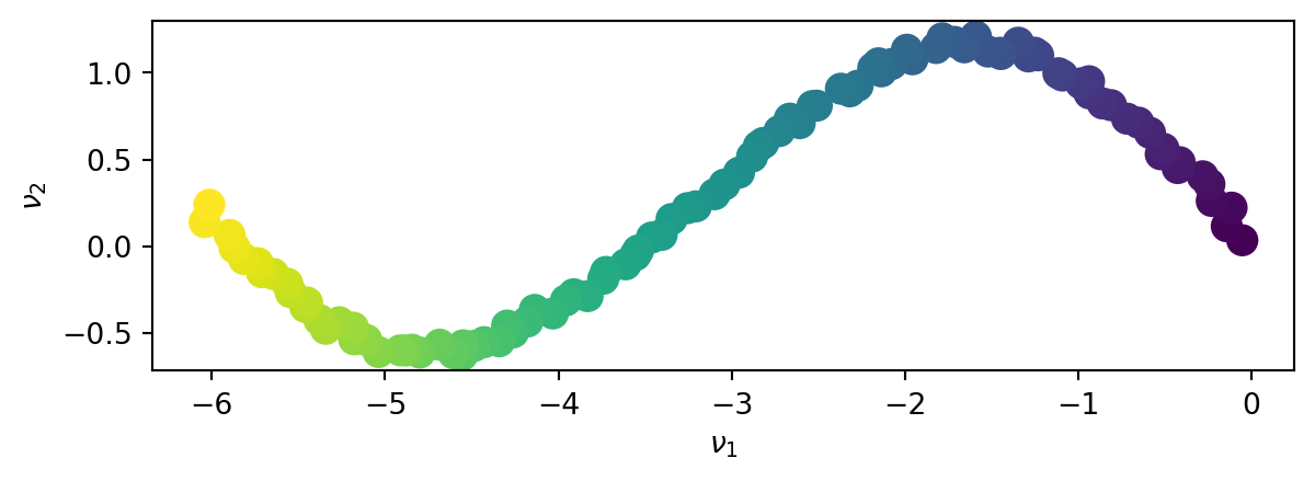

This time, the SVD does not exhibit a lower dimension space in which the data can be represented. Both principal directions are required to represent the non-linear data set.

kernel Principal Component Analysis (kPCA)

This section focuses on using using the kPCA to find a non-linear manifold of lower dimension in which to project the data. The objective is to show that dimensionality reduction works well in non-linear cases where the SVD failed.

Application to a sin function

We first apply the SVD to a sin function. The physical space of the dataset is \(\mathbb{R}3\) but the data set is in fact 2D. The kPCA is used to find a suitable 2D (non-linear) manifold in which the data can be projected without loosing any information.

Function definition

Code

x = np.linspace(0,4*np.pi,1500)
y = np.sin(x)                                                                   # Sin function
n_coef = 0                                                                      # Noise level
z = np.random.randn(*x.shape)        
X = np.stack((x,y,z))                                                           # Create 3D dataset
X += + n_coef*np.random.rand(*X.shape)                                          # Add noise

Note: The PCA conventions are transposed compared to SVD’s conventions

Code

Y = np.transpose(X)

kPCA parameters

We define the kPCA paramerets, namely

The number of components
\(\sigma\), the width of the kernel, controlling how much distant point are considered similar
- A smaller \(\sigma\) emphasises local structures, while a larger σσ captures more global patterns.

Code

n_components = 2                                                                 # Number of component of the kpca
sigma =100                                                                       # sigma for Gaussian kernel

Compute the (Gaussian) kernel

We now compute the kernel matrix based on the distance matrix using a Gaussian kernel

\[K(x_i, x_j) = \exp\left(-\frac{\|x_i - x_j\|^2}{2\sigma^2}\right)\]

Code

d_2 = np.sum(Y**2, axis=1).reshape(-1, 1) + np.sum(Y**2, axis=1) - 2 * np.dot(Y, Y.T)
K = np.exp(-d_2 / (2 * sigma**2))

Center the kernel matrix

We then center the kernel matrix as the PCA expects 0-mean data

\[ K_{\text{centered}} = K - \frac{1}{n} \mathbf{1} K - \frac{1}{n} K \mathbf{1} + \frac{1}{n^2} \mathbf{1} K \mathbf{1} \]

Code

n = K.shape[0]
one_n = np.ones((n, n)) / n
K_centered = K - one_n @ K - K @ one_n + one_n @ K @ one_n

We perform an SVD of the centered kernel to find the principal directions of the high dimensional space,

Code

U, S, V = np.linalg.svd(K_centered)

that we then truncates. we then project the initial dataset onto the principal directions in the latent space

Code

U_k = U[:, :n_components]  # first eigenvectors
S_k = np.diag(S[:n_components])  # first singular values
# Project the centered kernel matrix onto the first eigenvectors
Y_kpca = U_k @ S_k

Plots

In the physical space (the plot is interactive, feel free to explore the 3D dataset !)

Code

colors = plt.cm.viridis(np.linspace(0, 1, len(X[0,:])))                                        # Generate a color gradient

import plotly.graph_objects as go


# colors_plotly = colors[:, :3]
colors_plotly = np.linspace(0, 1, X.shape[1])

x_points = X[0, :]
y_points = X[1, :]
z_points = X[2, :]

# Create the 3D scatter plot
fig = go.Figure(data=[go.Scatter3d(
    x=x_points,
    y=y_points,
    z=z_points,
    mode='markers',
    marker=dict(
        size=5,                                                                         # Size of the markers
        color=colors_plotly,                                                            # Color of the markers
        colorscale='viridis',                                                           # Color scale
        showscale=True,                                                                 # Show color scale
    )
)])

fig.update_layout(
    scene=dict(
        xaxis_title='x',
        yaxis_title='y',
        zaxis_title='z',
    ),
    title='Physical Space'
)
fig.show()

In the latent space

Code

plt.scatter(Y_kpca[:,0], Y_kpca[:,1], color=colors, s=100)                                     # s=100 for larger points
plt.xlabel(r"$\nu_1$")
plt.ylabel(r"$\nu_2$")
plt.title('latent space')
plt.gca().set_aspect('equal', adjustable='box')
plt.show()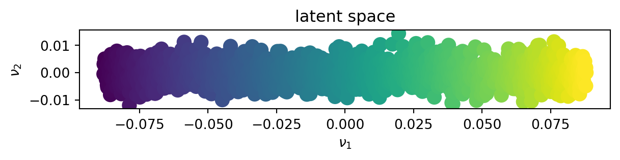

We can see that contrary to the SVD, the kPCA could decrease the dimensionnality of the supposidly 3D space into a 2D space, finding the underlying non-linear manifold onto which the dataset lies.

Application to a noisy affine function

We now apply the SVD to an affine function. The physical space of the dataset is still \(\mathbb{R}3\) but the data set is in fact 2D. The kPCA is used to find a suitable 2D linear subspace similarly to what the SVD would give.

Function definition

Code

x = np.linspace(0,4*np.pi,1500)
# Affine parameters
a = 1.5                                                                                     # Slope
b=0                                                                                         # y-axis origin

# Affine function
y = a*x+b 
n_coef = 1                                                                      # Noise level
z = np.random.randn(*x.shape)        
X = np.stack((x,y,z))                                                           # Create 3D dataset
X += + n_coef*np.random.rand(*X.shape)                                          # Add noise

Note: The PCA conventions are transposed compared to SVD’s conventions

Code

Y = np.transpose(X)

kPCA parameters

We define the kPCA paramerets, namely

The number of components
\(\sigma\), the width of the kernel, controlling how much distant point are considered similar
- A smaller \(\sigma\) emphasises local structures, while a larger \(\sigma\) captures more global patterns.

Code

n_components = 2                                                                 # Number of component of the kpca
sigma =100                                                                       # sigma for Gaussian kernel

Compute the (Gaussian) kernel

We now compute the kernel matrix based on the distance matrix using a Gaussian kernel

\[K(x_i, x_j) = \exp\left(-\frac{\|x_i - x_j\|^2}{2\sigma^2}\right)\]

Code

d_2 = np.sum(Y**2, axis=1).reshape(-1, 1) + np.sum(Y**2, axis=1) - 2 * np.dot(Y, Y.T)
K = np.exp(-d_2 / (2 * sigma**2))

Center the kernel matrix

We then center the kernel matrix as the PCA expects 0-mean data

\[ K_{\text{centered}} = K - \frac{1}{n} \mathbf{1} K - \frac{1}{n} K \mathbf{1} + \frac{1}{n^2} \mathbf{1} K \mathbf{1} \]

Code

n = K.shape[0]
one_n = np.ones((n, n)) / n
K_centered = K - one_n @ K - K @ one_n + one_n @ K @ one_n

We perform an SVD of the centered kernel to find the principal directions of the high dimensional space,

Code

U, S, V = np.linalg.svd(K_centered)

that we then truncates. we then project the initial dataset onto the principal directions in the latent space

Code

U_k = U[:, :n_components]  # first eigenvectors
S_k = np.diag(S[:n_components])  # first singular values
# Project the centered kernel matrix onto the first eigenvectors
Y_kpca = U_k @ S_k

Plots

In the physical space (the plot is interactive, feel free to explore the 3D dataset !)

Code

colors = plt.cm.viridis(np.linspace(0, 1, len(X[0,:])))                                        # Generate a color gradient

import plotly.graph_objects as go


# colors_plotly = colors[:, :3]
colors_plotly = np.linspace(0, 1, X.shape[1])

x_points = X[0, :]
y_points = X[1, :]
z_points = X[2, :]

# Create the 3D scatter plot
fig = go.Figure(data=[go.Scatter3d(
    x=x_points,
    y=y_points,
    z=z_points,
    mode='markers',
    marker=dict(
        size=5,                                                                         # Size of the markers
        color=colors_plotly,                                                            # Color of the markers
        colorscale='viridis',                                                           # Color scale
        showscale=True,                                                                 # Show color scale
    )
)])

fig.update_layout(
    scene=dict(
        xaxis_title='x',
        yaxis_title='y',
        zaxis_title='z',
    ),
    title='Physical Space'
)
fig.show()

In the latent space

Code

plt.scatter(Y_kpca[:,0], Y_kpca[:,1], color=colors, s=100)                                     # s=100 for larger points
plt.xlabel(r"$\nu_1$")
plt.ylabel(r"$\nu_2$")
plt.title('latent space')
plt.gca().set_aspect('equal', adjustable='box')
plt.show()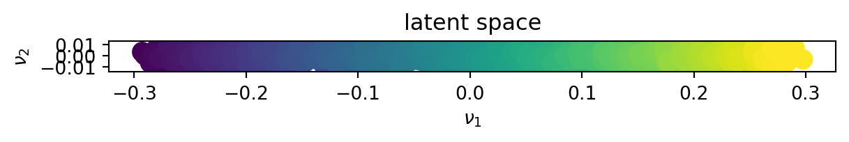

We can see that for linear data, the kPCA behaves similarly to the SVD.