Digital Twin of Human Lungs: Towards Real-Time Simulation and Registration of Soft Organs

ICCB 2025

Alexandre Daby-Seesaram

LMS, École Polytechnique, Paris, France

Katerina Skardova

LMS, École Polytechnique, Paris, France

Martin Genet

LMS, École Polytechnique, Paris, France

September 10, 2025

Idiopathic Pulmonary Fibrosis

Inspiration & expiration of diseased lungs

Digital twin from images

Objectives

  • Improved understanding of the mechanically-driven physiological mechanisms
  • In silico prognostics
    • Transfer tools to the clinic
    • Patient-specific digital twins

Requirements

  • Real-time estimation of the parameters

Simpler mechanical problem - surrogate modelling

  • Parametrised (patient-specific) mechanical problem

\[ \boldsymbol{u} = \mathop{\mathrm{arg\,min}}_{H^1\left(\Omega \right)} \int_{\Omega} \Psi\left( \boldsymbol{E}\left(\boldsymbol{u}\left(\textcolor{Blue}{\boldsymbol{x}}, \textcolor{LGreen}{\left\{\mu_i\right\}_{i \in \mathopen{~[\!\![~}1, \beta \mathclose{~]\!\!]}}}\right)\right) \right) ~\mathrm{d}\Omega- W_{\text{ext}}\left(\textcolor{Blue}{\boldsymbol{x}}, \textcolor{LGreen}{\left\{\mu_i\right\}_{i \in \mathopen{~[\!\![~}1, \beta \mathclose{~]\!\!]}}}\right) \]

Kinematics:

  • \(\boldsymbol{F} = \boldsymbol{1} + \boldsymbol{\nabla}\boldsymbol{u}\) - deformation gradient
  • \(\boldsymbol{C} = \boldsymbol{F}^T \cdot \boldsymbol{F}\) - right Cauchy-Green tensor
  • \(\boldsymbol{E} = \frac{1}{2}\left(\boldsymbol{C} -\boldsymbol{1} \right)\) - Green-Lagrange tensor
    • \(I_1 = \text{tr}\left(\boldsymbol{C} \right)\) - first invariant of \(\boldsymbol{C}\)

Behaviour - Saint Venant-Kirchhoff

\(\Psi = \frac{\lambda}{2} \text{tr}\left(\boldsymbol{E}\right)^2 + \mu \boldsymbol{E}:\boldsymbol{E}\)

  • Unstable under compression
  • \(\nu = 0.49\) for quasi-incompressibility
    • Soft tissues are often modelled as incompressible materials

Reduced-order model (ROM)

  • Build a surrogate model
    • Parametrised solution \(\left(\textcolor{Blue}{\boldsymbol{x}}, \textcolor{LGreen}{\left\{\mu_i\right\}_{i \in \mathopen{~[\!\![~}1, \beta \mathclose{~]\!\!]}}}\right)\)
  • No computations online
  • On the fly evaluation of the model
    • Real-time parameters estimation

Outline

  1. General Surrogate modelling methods and results
  1. Focus on patient-specific shape parametrisation

II - Methods

  1. Mechanical solution interpolation
  1. Reduced-order modelling
  1. Hybrid Neural Network Proper Generalised Decomposition
  1. Preliminary results

Interpolation of the solution

  • FEM finite admissible space

\[ \mathcal{U}_h = \left\{\boldsymbol{u}_h \; | \; \boldsymbol{u}_h \in \text{Span}\left( \left\{ N_i^{\Omega}\left(\boldsymbol{x} \right)\right\}_{i \in \mathopen{~[\!\![~}1,N\mathclose{~]\!\!]}} \right)^d \text{, } \boldsymbol{u}_h = \boldsymbol{u}_d \text{ on }\partial \Omega_d \right\} \]

  • Interpretabilty
  • Kronecker property
    • Easy to prescribe Dirichlet boundary conditions
  • Mesh adaptation not directly embedded in the method
  • Fully connected Neural Networks (e.g., PINNS)

\[ \boldsymbol{u} \left(x_{0,0,0} \right) = \sum\limits_{i = 0}^C \sum\limits_{j = 0}^{N_i} \sigma \left( \sum\limits_{k = 0}^{M_{i,j}} b_{i,j}+\omega_{i,j,k}~ x_{i,j,k} \right) \]

  • All interpolation parameters are trainable
  • Benefits from ML developments
  • Not easily interpretable
  • Difficult to prescribe Dirichlet boundary conditions
  • HiDeNN framework (Liu et al., 2023; Park et al., 2023; Zhang et al., 2021)
    • Best of both worlds
    • Reproducing FEM interpolation with constrained sparse neural networks
    • \(N_i^{\Omega}\) are SNN with constrained weights and biases
    • Fully interpretable parameters
    • Continuous interpolated field that can be automatically differentiated
    • Runs on GPUs

Illustration of the framework

Reduced-order modelling (ROM)

Low-rank approximation of the solution to avoid the curse of dimensionality with \(\beta\) parameters

Full-order discretised model

  • \(N\) spatial shape functions
    • Span a finite spatial space of dimension \(N\)
  • Requires computing \(N\times \beta\) associated parametric functions

Reduced-order model

  • \(m \ll N\) spatial modes
    • Similar to global shape functions
    • Span a smaller space
  • Galerkin projection

Finding the reduced-order basis

Proper Generalised Decomposition (PGD)

Tensor Decomposition

  • \(\textcolor{LGreen}{\textcolor{LGreen}{\left\{\mu_i\right\}_{i \in \mathopen{~[\!\![~}1, \beta \mathclose{~]\!\!]}}}}\) parameters (material, shape, loading, etc.)
  • Curse of dimensionality

\[ \textcolor{VioletLMS_2}{\boldsymbol{u}}\left(\textcolor{Blue}{\boldsymbol{x}}, \textcolor{LGreen}{\left\{\mu_i\right\}_{i \in \mathopen{~[\!\![~}1, \beta \mathclose{~]\!\!]}}}\right)\]

Discretised problem

3D PGD
  • \(\textcolor{VioletLMS_2}{N\times\prod\limits_{j=1}^{~\beta} N_{\mu}^j}\) unknowns
    • e.g. \(\textcolor{VioletLMS_2}{10000 \times 1000^2 = 10^{10}}\)

Proper Generalised Decomposition (PGD)

Tensor Decomposition

  • \(\textcolor{LGreen}{\textcolor{LGreen}{\left\{\mu_i\right\}_{i \in \mathopen{~[\!\![~}1, \beta \mathclose{~]\!\!]}}}}\) parameters (material, shape, loading, etc.)
  • Curse of dimensionality

\[ \textcolor{VioletLMS_2}{\boldsymbol{u}}\left(\textcolor{Blue}{\boldsymbol{x}}, \textcolor{LGreen}{\left\{\mu_i\right\}_{i \in \mathopen{~[\!\![~}1, \beta \mathclose{~]\!\!]}}}\right) = \sum\limits_{i=1}^m \textcolor{Blue}{\overline{\boldsymbol{u}}_i(\boldsymbol{x})} ~\textcolor{LGreen}{\prod_{j=1}^{\beta}\lambda_i^j(\mu^j)}\]

  • \(\textcolor{Blue}{\overline{\boldsymbol{u}}_i(\boldsymbol{x})}\) space modes
  • \(\textcolor{LGreen}{\lambda_i^j(\mu^j)}\) parameter modes

Discretised problem

3D PGD
  • From \(\textcolor{VioletLMS_2}{N\times\prod\limits_{j=1}^{~\beta} N_{\mu}^j}\) unknowns to \(\textcolor{Blue}{m\times\left(N + \sum\limits_{j=1}^{\beta} N_{\mu}^j\right)}\)
    • e.g. \(\textcolor{VioletLMS_2}{10000 \times 1000^2 = 10^{10}} \gg \textcolor{Blue}{ 5\left( 10 000+ 2\times 1000 \right) = 6 \times 10^4}\)
  • Finding the tensor decomposition by minimising the energy \[ \left(\left\{\overline{\boldsymbol{u}}_i \right\}_{i\in \mathopen{~[\!\![~}1,m\mathclose{~]\!\!]}},\left\{\lambda_i^j \right\}_{ \begin{cases} i\in \mathopen{~[\!\![~}1,m\mathclose{~]\!\!]}\\ j\in \mathopen{~[\!\![~}1,\beta \mathclose{~]\!\!]} \end{cases} } \right) = \mathop{\mathrm{arg\,min}}_{ \begin{cases} \left(\overline{\boldsymbol{u}}_1, \left\{\overline{\boldsymbol{u}}_i \right\} \right) & \in \mathcal{U}\times \mathcal{U}_0 \\ \left\{\left\{\lambda_i^j \right\}\right\} & \in \left( \bigtimes_{j=1}^{~\beta} \mathcal{L}_2\left(\mathcal{B}_j\right) \right)^{m-1} \end{cases}} ~\underbrace{\int_{\mathcal{B}}\left[E_p\left(\boldsymbol{u}\left(\boldsymbol{x},\left\{\mu_i\right\}_{i \in \mathopen{~[\!\![~}1, \beta \mathclose{~]\!\!]}}\right), \mathbb{C}, \boldsymbol{F}, \boldsymbol{f} \right) \right]\mathrm{d}\beta}_{\mathcal{L}} \label{eq:min_problem} \]

Proper Generalised Decomposition (PGD)

\[ \boldsymbol{u}\left(\boldsymbol{x}, \left\{\mu_i\right\}_{i \in \mathopen{~[\!\![~}1, \beta \mathclose{~]\!\!]}}\right) = \overline{\boldsymbol{u}}(\boldsymbol{x}) ~\prod_{j=1}^{\beta}\lambda^j(\mu^j) \]

\[ \boldsymbol{u}\left(\boldsymbol{x}, \left\{\mu_i\right\}_{i \in \mathopen{~[\!\![~}1, \beta \mathclose{~]\!\!]}}\right) = \textcolor{red}{\sum\limits_{i=1}^{2}} \overline{\boldsymbol{u}}_{\textcolor{red}{i}}(\boldsymbol{x}) ~\prod_{j=1}^{\beta}\lambda_{\textcolor{red}{i}}^j(\mu^j) \]

\[ \boldsymbol{u}\left(\boldsymbol{x}, \left\{\mu_i\right\}_{i \in \mathopen{~[\!\![~}1, \beta \mathclose{~]\!\!]}}\right) = \sum\limits_{i=1}^{\textcolor{red}{m}} \overline{\boldsymbol{u}}_i(\boldsymbol{x}) ~\prod_{j=1}^{\beta}\lambda_i^j(\mu^j) \]

Greedy algorithm

  1. Start with a single mode
  2. Minimise the loss until stagnation
  1. Add a new mode
  2. If loss decreases, continue training
  1. Else stop and return the converged model

The PGD is

  • An a priori ROM techniques
    • Building the model from scratch on the fly
  • No full-order computations
  • Reduced-order basis tailored to the specifics of the problem (Daby-Seesaram et al., 2023)

Note

  • Training of the full tensor decomposition, not only the \(m\)-th mode
  • Actual minimisation implementation of the PGD
  • No need to solve a new problem for any new parameter
    • The online stage is a simple evaluation of the tensor decomposition

Neural Network PGD

Graphical implementation of Neural Network PGD

\[ \boldsymbol{u}\left(\textcolor{Blue}{\boldsymbol{x}}, \textcolor{LGreen}{\left\{\mu_i\right\}_{i \in \mathopen{~[\!\![~}1, \beta \mathclose{~]\!\!]}}}\right) = \sum\limits_{i=1}^m \textcolor{Blue}{\overline{\boldsymbol{u}}_i(\boldsymbol{x})} ~\textcolor{LGreen}{\prod_{j=1}^{\beta}\lambda_i^j(\mu^j)} \]

Interpretable NN-PGD

  • No black box
    • Fully interpretable implementation
    • Great transfer learning capabilities
  • Straightforward implementation
    • Benefiting from current ML developments
  • Straightforward definition of the physical loss using auto-differentiation
def Loss(model,x,detJ,mu):
  
    u = model.space_mode(x)
    eps = torch.autograd.grad(u, x, grad_outputs=torch.ones_like(u))
    lmbda = model.parameter_mode(mu)
    W_int = torch.einsum('ij,ejm,eil,em,mp...,lp...,p->',C,eps,eps,detJ,lmbda,lmbda, mu)

    return 0.5*W_int/mu.shape[0]

NN-PGD

Stiffness and external forces parametrisation

Illustration of the surrogate model in use (Daby-Seesaram et al., 2025)

Mechanical problem 2D

Parameters

  • Parametrised stiffness \(E\)
  • Parametrised external force \(\boldsymbol{f} = \begin{bmatrix} ~ \rho g \sin\left( \theta \right) \\ -\rho g \cos\left( \theta \right) \cos\left( \phi \right) \\ \rho g \cos\left( \theta \right) \sin\left( \phi \right) \end{bmatrix}\)

NeuROM

NN-PGD

  • Immediate evaluation of the surrogate model (~100Hz)
  • Straightforward differentiation capabilities regarding the input parameters

Convergence of the greedy algorithm

Loss convergence

Loss decay

Construction of the ROB

  • New modes are added when the loss’s decay cancels out
  • Adding a new mode gives extra latitude to improve predictivity

Accuracy with regards to FEM solutions

Solution Error
Configuration 1
\(E = 3.8 \times 10^{-3}\mathrm{ MPa}, \theta = 241^\circ\)
Configuration 1 Error
\(E = 3.8 \times 10^{-3}\mathrm{ MPa}, \theta = 241^\circ\)
Configuration 2
\(E = 3.1 \times 10^{-3}\mathrm{ MPa}, \theta = 0^\circ\)
Configuration 2 Error
\(E = 3.1 \times 10^{-3}\mathrm{ MPa}, \theta = 0^\circ\)
\(E\) (kPa) \(\theta\) (rad) Relative error
3.80 1.57 \(1.12 \times 10^{-3}\)
3.80 4.21 \(8.72 \times 10^{-4}\)
3.14 0 \(1.50 \times 10^{-3}\)
4.09 3.70 \(8.61 \times 10^{-3}\)
4.09 3.13 \(9.32 \times 10^{-3}\)
4.62 0.82 \(2.72 \times 10^{-3}\)
5.01 2.26 \(5.35 \times 10^{-3}\)
6.75 5.45 \(1.23 \times 10^{-3}\)

Multi-level training

Multi-level training convergence

Strategy

  • The interpretability of the NN allows
    • Great transfer learning capabilities
      • Start with coarse (cheap) training
      • Followed by fine tuning, refining all modes
  • Extends the idea put forward by (Giacoma et al., 2015)

Note

  • The structure of the Tensor decomposition is kept throughout the multi-level training
  • Last mode of each level is irrelevant by construction
    • It is removed before passing onto the next refinement level

III - Patient-specific parametrisation

  1. Shape registration pipeline from CT-scans
  1. Building a geometry model from the shapes library

AR model

Shape model - parametrisation

Encoding the shape of the lung in a low-dimensional space

  • In order to feed the surrogate model we need a parametrisation of the lung
  • ROM on the shape mappings library
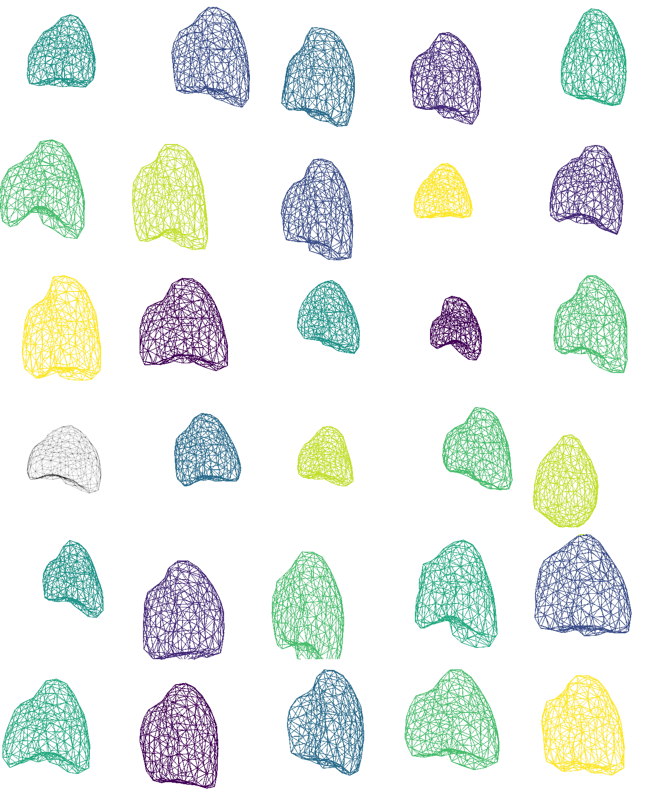
Mappings’ library

Mappings’ library

Shape model

  • Shape analysis
  • Model-order reduction on shapes
    • Parametrisation of the shape
    • \(\Omega = \Omega\left(\textcolor{LGreenLMS}{\left\{\mu_i\right\}_{i \in \mathopen{~[\!\![~}1, \beta \mathclose{~]\!\!]}}}\right)\)
      • SVD
      • k-PCA
      • Auto-encoder
    • Personalising the digital twin

Conclusion

Conclusion

  • Robust and straightforward general implementation of a NN-PGD
    • Interpretable
    • Benefits from all recent developments in machine learning
  • Surrogate modelling of parametrised PDE solution
    • Promising results on simple toy case

Perspectives for patient-specific applications

  • Implementation of the poro-mechanics lung model (Patte et al., 2022)
  • Further work on parametrising the geometries
  • Inputting geometry parameters in the NN-PGD
  • Error quantification on the estimated parameters

Technical perspectives

  • Stochastic integration (curse of dimensionality for non-separable quantities)
  • Non-linear reduced order modelling
  • Do not hesitate to check the Github page

References

Barrault, M., Maday, Y., Nguyen, N. C., & Patera, A. T. (2004). An “empirical interpolation” method: Application to efficient reduced-basis discretization of partial differential equations. Comptes Rendus Mathematique, 339(9), 667–672. https://doi.org/10.1016/j.crma.2004.08.006
Chatterjee, A. (2000). An introduction to the proper orthogonal decomposition. Current Science, 78(7), 808–817. https://www.jstor.org/stable/24103957
Chinesta, F., Ladeveze, P., & Cueto, E. (2011). A Short Review on Model Order Reduction Based on Proper Generalized Decomposition. Archives of Computational Methods in Engineering, 18(4), 395–404. https://doi.org/10.1007/s11831-011-9064-7
Daby-Seesaram, A., Fau, A., Charbonnel, P.-É., & Néron, D. (2023). A hybrid frequency-temporal reduced-order method for nonlinear dynamics. Nonlinear Dynamics, 111(15), 13669–13689. https://doi.org/10.1007/s11071-023-08513-8
Daby-Seesaram, A., Škardová, K., & Genet, M. (2025). Finite element neural network interpolation: Part II—hybridisation with the proper generalised decomposition for non-linear surrogate modelling. Computational Mechanics. https://doi.org/10.1007/s00466-025-02676-4
Gangl, P., Sturm, K., Neunteufel, M., & Schöberl, J. (2021). Fully and semi-automated shape differentiation in NGSolve. Structural and Multidisciplinary Optimization, 63(3), 1579–1607. https://doi.org/10.1007/s00158-020-02742-w
Giacoma, A., Dureisseix, D., Gravouil, A., & Rochette, M. (2015). Toward an optimal a priori reduced basis strategy for frictional contact problems with LATIN solver. Computer Methods in Applied Mechanics and Engineering, 283, 1357–1381. https://doi.org/10.1016/j.cma.2014.09.005
Hansteen, O. E., & Bell, K. (1979). On the accuracy of mode superposition analysis in structural dynamics. Earthquake Engineering & Structural Dynamics, 7(5), 405–411. https://doi.org/10.1002/eqe.4290070502
Ladeveze, P. (1985). Sur une famille d’algorithmes en mécanique des structures. Sur Une Famille d’algorithmes En Mécanique Des Structures, 300(2), 41–44.
Laville, C., Fetita, C., Gille, T., Brillet, P.-Y., Nunes, H., Bernaudin, J.-F., & Genet, M. (2023). Comparison of optimization parametrizations for regional lung compliance estimation using personalized pulmonary poromechanical modeling. Biomechanics and Modeling in Mechanobiology, 22(5), 1541–1554. https://doi.org/10.1007/s10237-023-01691-9
Liu, Y., Park, C., Lu, Y., Mojumder, S., Liu, W. K., & Qian, D. (2023). HiDeNN-FEM: A seamless machine learning approach to nonlinear finite element analysis. Computational Mechanics, 72(1), 173–194. https://doi.org/10.1007/s00466-023-02293-z
Maday, Y., & Rønquist, E. M. (2002). A Reduced-Basis Element Method. Journal of Scientific Computing, 17(1), 447–459. https://doi.org/10.1023/A:1015197908587
Neuberger, J. W. (1985). Steepest descent and differential equations. Journal of the Mathematical Society of Japan, 37(2), 187–195. https://doi.org/10.2969/jmsj/03720187
Neuberger, J. W. (1997). Sobolev Gradients and Differential Equations (Vol. 1670). Springer. https://doi.org/10.1007/BFb0092831
Nouy, A. (2010). A priori model reduction through Proper Generalized Decomposition for solving time-dependent partial differential equations. Computer Methods in Applied Mechanics and Engineering, 199(23–24), 1603–1626. https://doi.org/10.1016/j.cma.2010.01.009
Park, C., Lu, Y., Saha, S., Xue, T., Guo, J., Mojumder, S., Apley, D. W., Wagner, G. J., & Liu, W. K. (2023). Convolution hierarchical deep-learning neural network (C-HiDeNN) with graphics processing unit (GPU) acceleration. Computational Mechanics, 72(2), 383–409. https://doi.org/10.1007/s00466-023-02329-4
Patte, C., Genet, M., & Chapelle, D. (2022). A quasi-static poromechanical model of the lungs. Biomechanics and Modeling in Mechanobiology, 21(2), 527–551. https://doi.org/10.1007/s10237-021-01547-0
Peyraut, A., & Genet, M. (2024). Quantification d’incertitudes pour la modélisation pulmonaire per- sonnalisée.
Peyraut, A., & Genet, M. (2025). Uncertainty quantification for personalized biomechanical modeling: Application to pulmonary poromechanical digital twins. Journal of Biomechanical Engineering.
Radermacher, A., & Reese, S. (2013). A comparison of projection-based model reduction concepts in the context of nonlinear biomechanics. Archive of Applied Mechanics, 83(8), 1193–1213. https://doi.org/10.1007/s00419-013-0742-9
Škardová, K., Daby-Seesaram, A., & Genet, M. (2025). Finite element neural network interpolation: Part I—interpretable and adaptive discretization for solving PDEs. Computational Mechanics. https://doi.org/10.1007/s00466-025-02677-3
Zhang, L., Cheng, L., Li, H., Gao, J., Yu, C., Domel, R., Yang, Y., Tang, S., & Liu, W. K. (2021). Hierarchical deep-learning neural networks: Finite elements and beyond. Computational Mechanics, 67(1), 207–230. https://doi.org/10.1007/s00466-020-01928-9