Finite Element Neural Network Interpolation: Hybridisation with the Proper Generalised Decomposition for Surrogate Modelling
DTE & AICOMAS 2025
February 21, 2025
Interpolation of the solution
- FEM finite admissible space
\[ \mathcal{U}_h = \left\{\boldsymbol{u}_h \; | \; \boldsymbol{u}_h \in \text{Span}\left( \left\{ N_i^{\Omega}\left(\boldsymbol{x} \right)\right\}_{i \in \mathopen{~[\!\![~}1,N\mathclose{~]\!\!]}} \right)^d \text{, } \boldsymbol{u}_h = \boldsymbol{u}_d \text{ on }\partial \Omega_d \right\} \]
Interpretabilty Kronecker property Easy to prescribe Dirichlet boundary conditions
Mesh adaptation not directly embedded in the method
- Physics Informed Neural Networks (PINNs)
\[ \boldsymbol{u} \left(x_{0,0,0} \right) = \sum\limits_{i = 0}^C \sum\limits_{j = 0}^{N_i} \sigma \left( \sum\limits_{k = 0}^{M_{i,j}} b_{i,j}+\omega_{i,j,k}~ x_{i,j,k} \right) \]
All interpolation parameters are trainable Benefits from ML developments
Not easily interpretable Difficult to prescribe Dirichlet boundary conditions
- HiDeNN framework (Liu et al., 2023; Park et al., 2023; Zhang et al., 2021)
- Best of both worlds
- Reproducing FEM interpolation with constrained sparse neural networks
- \(N_i^{\Omega}\) are SNN with constrained weights and biases
- Fully interpretable parameters
- Continuous interpolated field that can be automatically differentiated
- Runs on GPUs

Proper Generalised Decomposition (PGD)
PGD: (Chinesta et al., 2011; Ladeveze, 1985)
Tensor decomposition
- Separation of variables
- Low-rank \(m\)
- \(\textcolor{BleuLMPS}{\overline{\boldsymbol{u}}_i(\boldsymbol{x})}\) Space modes
- \(\textcolor{LGreenLMS}{\lambda_i^j(\mu^j)}\) Parameter modes
\[\textcolor{VioletLMS}{\boldsymbol{u}}\left(\textcolor{BleuLMPS}{\boldsymbol{x}}, \textcolor{LGreenLMS}{\mu}\right) = \sum\limits_{i=0}^{m}\textcolor{BleuLMPS}{\overline{u}_i\left(x\right)}\textcolor{LGreenLMS}{\lambda_i\left(\mu\right)}\]
Discretised problem

- From \(N\times N_{\mu}\) unknowns to \(m\times\left(N + N_{\mu}\right)\)
- e.g. \(10000 \times 1000 = 1e7 \gg 5\left( 10 000+ 1000 \right) = 5.5e4\)
Proper Generalised Decomposition (PGD)
PGD: (Chinesta et al., 2011; Ladeveze, 1985)
Tensor decomposition - extra-coordinates
- Separation of variables
- Low-rank \(m\)
- \(\textcolor{BleuLMPS}{\overline{\boldsymbol{u}}_i(\boldsymbol{x})}\) Space modes
- \(\textcolor{LGreenLMS}{\lambda_i^j(\mu^j)}\) Parameter modes
\[ \textcolor{VioletLMS}{\boldsymbol{u}}\left(\textcolor{BleuLMPS}{\boldsymbol{x}}, \textcolor{LGreenLMS}{\left\{\mu_i\right\}_{i \in \mathopen{~[\!\![~}1, \beta \mathclose{~]\!\!]}}}\right) = \sum\limits_{i=1}^m \textcolor{BleuLMPS}{\overline{\boldsymbol{u}}_i(\boldsymbol{x})} ~\textcolor{LGreenLMS}{\prod_{j=1}^{\beta}\lambda_i^j(\mu^j)} \]
Discretised problem

- From \(N\times\prod\limits_{j=1}^{~\beta} N_{\mu}^j\) unknowns to \(m\times\left(N + \sum\limits_{j=1}^{\beta} N_{\mu}^j\right)\)
- e.g. \(10000 \times 1000^2 = 1e10 \gg 5\left( 10 000+ 2\times 1000 \right) = 6e4\)
- Finding the tensor decomposition by minimising the energy \[ \left(\left\{\overline{\boldsymbol{u}}_i \right\}_{i\in \mathopen{~[\!\![~}1,m\mathclose{~]\!\!]}},\left\{\lambda_i^j \right\}_{ \begin{cases} i\in \mathopen{~[\!\![~}1,m\mathclose{~]\!\!]}\\ j\in \mathopen{~[\!\![~}1,\beta \mathclose{~]\!\!]} \end{cases} } \right) = \mathop{\mathrm{arg\,min}}_{ \begin{cases} \left(\overline{\boldsymbol{u}}_1, \left\{\overline{\boldsymbol{u}}_i \right\} \right) & \in \mathcal{U}\times \mathcal{U}_0 \\ \left\{\left\{\lambda_i^j \right\}\right\} & \in \left( \bigtimes_{j=1}^{~\beta} \mathcal{L}_2\left(\mathcal{B}_j\right) \right)^{m-1} \end{cases}} ~\underbrace{\int_{\mathcal{B}}\left[E_p\left(\boldsymbol{u}\left(\boldsymbol{x},\left\{\mu_i\right\}_{i \in \mathopen{~[\!\![~}1, \beta \mathclose{~]\!\!]}}\right), \mathbb{C}, \boldsymbol{F}, \boldsymbol{f} \right) \right]\mathrm{d}\beta}_{\mathcal{L}} \label{eq:min_problem} \]
Neural Network PGD
Graphical implementation of Neural Network PGD
\[ \boldsymbol{u}\left(\textcolor{BleuLMPS}{\boldsymbol{x}}, \textcolor{LGreenLMS}{\left\{\mu_i\right\}_{i \in \mathopen{~[\!\![~}1, \beta \mathclose{~]\!\!]}}}\right) = \sum\limits_{i=1}^m \textcolor{BleuLMPS}{\overline{\boldsymbol{u}}_i(\boldsymbol{x})} ~\textcolor{LGreenLMS}{\prod_{j=1}^{\beta}\lambda_i^j(\mu^j)} \]
Interpretable NN-PGD
- No black box
- Fully interpretable implementation
- Great transfer learning capabilities
- Straightforward implementation
- Benefiting from current ML developments
- Straightforward definition of the physical loss using auto-differentiation

Stiffness and external forces parametrisation
Illustration of the surrogate model in use (preprint: Daby-Seesaram et al., 2024)

Parameters
- Parametrised stiffness \(E\)
- Parametrised external force \(\boldsymbol{f} = \begin{bmatrix} ~ \rho g \sin\left( \theta \right) \\ -\rho g \cos\left( \theta \right) \end{bmatrix}\)
NN-PGD
- Immediate evaluation of the surrogate model
- Straightforward differentiation capabilities regarding the input parameters
Accuracy with regards to FEM solutions
| Solution | Error |
|---|---|
 \(E = 3.8 \times 10^{-3}\mathrm{ MPa}, \theta = 241^\circ\) |
 \(E = 3.8 \times 10^{-3}\mathrm{ MPa}, \theta = 241^\circ\) |
 \(E = 3.1 \times 10^{-3}\mathrm{ MPa}, \theta = 0^\circ\) |
 \(E = 3.1 \times 10^{-3}\mathrm{ MPa}, \theta = 0^\circ\) |
| \(E\) (kPa) | \(\theta\) (rad) | Relative error |
|---|---|---|
| 3.80 | 1.57 | \(1.12 \times 10^{-3}\) |
| 3.80 | 4.21 | \(8.72 \times 10^{-4}\) |
| 3.14 | 0 | \(1.50 \times 10^{-3}\) |
| 4.09 | 3.70 | \(8.61 \times 10^{-3}\) |
| 4.09 | 3.13 | \(9.32 \times 10^{-3}\) |
| 4.62 | 0.82 | \(2.72 \times 10^{-3}\) |
| 5.01 | 2.26 | \(5.35 \times 10^{-3}\) |
| 6.75 | 5.45 | \(1.23 \times 10^{-3}\) |
Multi-level training

Strategy
- The interpretability of the NN allows
- Great transfer learning capabilities
- Start with coarse (cheap) training
- Followed by fine tuning, refining all modes
- Great transfer learning capabilities
- Extends the idea put forward by (Giacoma et al., 2015)
Note
- The structure of the Tensor decomposition is kept throughout the multi-level training
- Last mode of each level is irrelevant by construction
- It is removed before passing onto the next refinement level
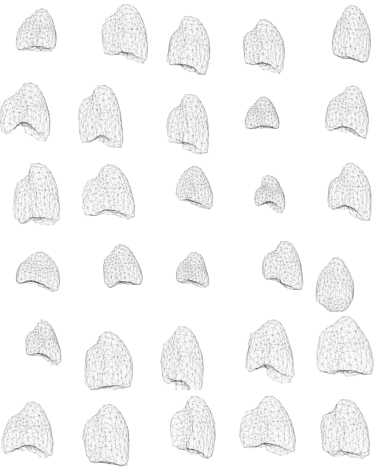
III - Patient-specific parametrisation
|
|

Shape model - parametrisation
Encoding the shape of the lung in low-dimensional spaces
- in order to feed the surrogate model we need a parametrisation of the lung
- ROM on the shape mappings librairy
Conclusion
Conclusion
- Robust and straightforward general implementation of a NN-PGD
- Interpretable
- Benefits from all recent developments in machine learning
- Surrogate modelling of parametrised PDE solution
- Promising results on simple toy case
Perspectives for patient-specific applications
- Implementation of the poro-mechanics lung model (Patte et al., 2022)
- Further work on parametrising the geometries
- Inputting geometry parameters in the NN-PGD
- Error quantification on the estimated parameters
Technical perspectives
- 3D implementation
- Seamless coupling of both tools
- Do not hesitate to check the Github page


Heterogeneous stiffness
- Bi-stiffness structure with unknown
- Stiffness jump \(\Delta E\)
- Jump position \(\alpha\)
- Towards the parametrisation of the disease’s progression
- Can be adapted to different stages of the diseases
- Different physiological initial stiffness


Heterogeneous stiffness
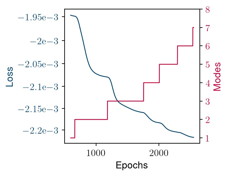
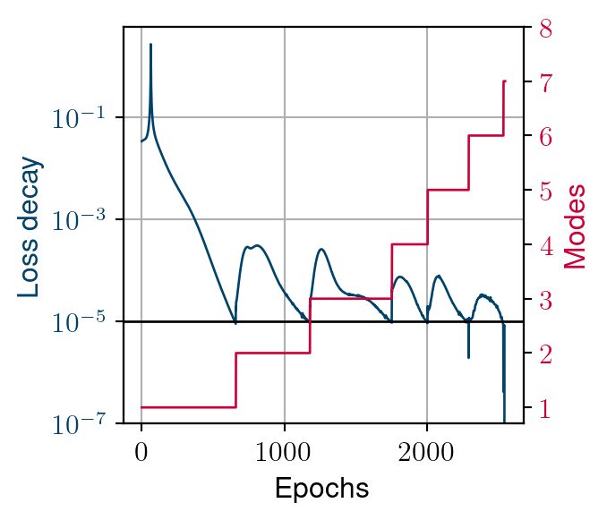
Convergence process
- Larger Kolmogorov n-with’s example
- Similar behaviour in constructing the reduced-order basis
- Adding a mode leads to a recovery in loss decay
- This recovery decreases until global stagnation
Hybridising ROM with NN

Shape model - registration (Gangl et al., 2021)
Minimisation problem
- The objective is to find the domain \(\omega\) occupied by a given segmented shape in a 3D image
- Which is solution of
\[\omega = \arg \min\underbrace{ \int_{\omega} I\left( x \right) \mathrm{d}\omega}_{\Psi\left(\omega\right)}\]
With requirement that \(I\left( x \right) \begin{cases} < 0 \forall x \in \mathcal{S} \\ > 0 \forall x \not \in \mathcal{S} \end{cases}\), with \(\mathcal{S}\) the image footprint of the shape to be registered
The domain \(\omega\) can be described by mapping \[\Phi\left(X\right) = I_d + u\left(X\right)\] from a reference shape \(\Omega\), leading to \[\int_{\omega} I\left( x \right) \mathrm{d}\omega = \int_{\Omega} I \circ \Phi \left( X \right) J \mathrm{d}\Omega\]
Shape derivatives
\(D\Psi\left(\omega\right)\left(\boldsymbol{u}^*\right) = \int_{\Omega} \nabla I \cdot u^* J \mathrm{d}\Omega + \underbrace{\int_{\Omega}I \circ \Phi\left(X\right) (F^T)^{-1} : \nabla u^* J \mathrm{d}\Omega}_{\int_{\omega}I\left(x\right) \mathrm{div}\left( u^* \circ \Phi \right) \mathrm{d}\omega}\)
Note that \[\int_{\omega}I\left(x\right) \mathrm{div}\left( u^* \circ \Phi \right) \mathrm{d}\omega = \int_{\partial \omega} I u^* \cdot n \partial \omega\]
Flat parts of the image result in non-zero derivative of the loss - The border is “pushed in the right direction”
Sobolev gradient (Neuberger, 1985; Neuberger, 1997)
- The regularisation is added through the choice of inner product \(H\) to reconstruct the gradient
\[D\Psi\left(u\right)\left(v^*\right) = \left(\nabla^H \Psi \left(u\right), v^* \right)_H\]
- Classically:
- \(\left(\boldsymbol{u}, \boldsymbol{v}^* \right)_H := \int_{\omega} \boldsymbol{\nabla_s}\boldsymbol{u}:\boldsymbol{\nabla_s}\boldsymbol{\boldsymbol{v}^*}\mathrm{d}\omega + \alpha \int_{\omega} \boldsymbol{u} \cdot \boldsymbol{v^*}\mathrm{d}\omega\)
![]()